Introduction to PyTorch and Poutyne

Note

• See the notebook here

• Run in Google Colab

In this example, we train a simple fully-connected network and a simple convolutional network on MNIST. First, we train it by coding our own training loop as the PyTorch library expects of us to. Then, we use Poutyne to simplify our code.

Let’s import all the needed packages.

import os
import math

import matplotlib.pyplot as plt
import numpy as np
import torch
import torch.nn as nn
import torch.optim as optim
from torch.utils.data import random_split, DataLoader
from torchvision import transforms, utils
from torchvision.datasets.mnist import MNIST

from poutyne import set_seeds, Model, ModelCheckpoint, CSVLogger, ModelBundle

Also, we need to set Pythons’s, NumPy’s and PyTorch’s seeds by using Poutyne function so that our training is (almost) reproducible.

set_seeds(42)

Basis of Training a Neural Network

In stochastic gradient descent, a batch of m examples are drawn from the train dataset. In the so-called forward pass, these examples are passed through the neural network and an average of their loss values is done. In the backward pass, the average loss is backpropagated through the network to compute the gradient of each parameter. In practice, the m examples of a batch are drawn without replacement. Thus, we define one epoch of training being the number of batches needed to loop through the entire training dataset.

In addition to the training dataset, a validation dataset is used to evaluate the neural network at the end of each epoch. This validation dataset can be used to select the best model during training and thus avoiding overfitting the training set. It also can have other uses such as selecting hyperparameters

Finally, a test dataset is used at the end to evaluate the final model.

Training constants

Now, let’s set our training constants. We first have the CUDA device used for training if one is present. Second, we set the train_split to 0.8 (80%) to use 80% of the dataset for training and 20% for validation. Third, we set the number of classes (i.e. one for each number). Finally, we set the batch size (i.e. the number of elements to see before updating the model), the learning rate for the optimizer, and the number of epochs (i.e. the number of times we see the full dataset).

cuda_device = 0
device = torch.device("cuda:%d" % cuda_device if torch.cuda.is_available() else "cpu")

train_split_percent = 0.8

num_classes = 10

batch_size = 32
learning_rate = 0.1
num_epochs = 5

Loading the MNIST dataset

The following loads the MNIST dataset and creates the PyTorch DataLoaders that split our datasets into batches. The train DataLoader shuffles the examples of the train dataset to draw the examples without replacement.

full_train_dataset = MNIST('./datasets/', train=True, download=True, transform=transforms.ToTensor())
test_dataset = MNIST('./datasets/', train=False, download=True, transform=transforms.ToTensor())

num_data = len(full_train_dataset)
train_length = int(math.floor(train_split_percent * num_data))
valid_length = num_data - train_length

train_dataset, valid_dataset = random_split(
    full_train_dataset,
    [train_length, valid_length],
    generator=torch.Generator().manual_seed(42),
)

train_loader = DataLoader(train_dataset, batch_size=batch_size, num_workers=2, shuffle=True)
valid_loader = DataLoader(valid_dataset, batch_size=batch_size, num_workers=2)
test_loader = DataLoader(test_dataset, batch_size=batch_size, num_workers=2)

loaders = train_loader, valid_loader, test_loader

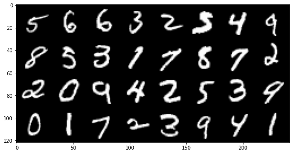
Let’s look at some examples of the dataset by looking at the first batch in our train DataLoader and formatting it into a grid and plotting it.

inputs = next(iter(train_loader))[0]
input_grid = utils.make_grid(inputs)

fig = plt.figure(figsize=(10, 10))
inp = input_grid.numpy().transpose((1, 2, 0))
plt.imshow(inp)
plt.show()

Here the resulting image

Neural Network Architectures

We train a fully-connected neural network and a convolutional neural network with approximately the same number of parameters.

Fully-connected Network

In short, the fully-connected network follows this architecture: Input -> [Linear -> ReLU]*3 -> Linear. The following table shows it in details:

Layer Type	Output size	# of Parameters
Input	1x28x28	0
Flatten	1*28*28	0
Linear with 256 neurons	256	28*28*256 + 256 = 200,960
ReLU	*	0
Linear with 128 neurons	128	256*128 + 128 = 32,896
ReLU	*	0
Linear with 64 neurons	64	128*64 + 64 = 8,256
ReLU	*	0
Linear with 10 neurons	10	64*10 + 10 = 650

Total # of parameters of the fully-connected network: 242,762

Convolutional Network

The convolutional neural network architecture starts with some convolution and max-pooling layers. These are then followed by fully-connected layers. We calculate the total number of parameters that the network needs. In short, the convolutional network follows this architecture: Input -> [Conv -> ReLU -> MaxPool]*2 -> Dropout -> Linear -> ReLU -> Dropout -> Linear. The following table shows it in details:

Layer Type	Output Size	# of Parameters
Input	1x28x28	0
Conv with 16 3x3 filters with padding of 1	16x28x28	16*1*3*3 + 16 = 160
ReLU	16x28x28	0
MaxPool 2x2	16x14x14	0
Conv with 32 3x3 filters with padding of 1	32x14x14	32*16*3*3 + 32 = 4,640
ReLU	32x14x14	0
MaxPool 2x2	32x7x7	0
Dropout of 0.25	32x7x7	0
Flatten	32*7*7	0
Linear with 128 neurons	128	32*7*7*128 + 128 = 200,832
ReLU	128	0
Dropout of 0.5	128	0
Linear with 10 neurons	10	128*10 + 10 = 1290

Total # of parameters of the convolutional network: 206,922

def create_fully_connected_network():
    """
    This function returns the fully-connected network layed out above.
    """
    return nn.Sequential(
        nn.Flatten(),
        nn.Linear(28*28, 256),
        nn.ReLU(),
        nn.Linear(256, 128),
        nn.ReLU(),
        nn.Linear(128, 64),
        nn.ReLU(),
        nn.Linear(64, num_classes)
    )

def create_convolutional_network():
    """
    This function returns the convolutional network layed out above.
    """
    return nn.Sequential(
        nn.Conv2d(in_channels=1, out_channels=16, kernel_size=3, padding=1),
        nn.ReLU(),
        nn.MaxPool2d(2),
        nn.Conv2d(in_channels=16, out_channels=32, kernel_size=3, padding=1),
        nn.ReLU(),
        nn.MaxPool2d(2),
        nn.Dropout(0.25),
        nn.Flatten(),
        nn.Linear(32*7*7, 128),
        nn.ReLU(),
        nn.Dropout(0.5),
        nn.Linear(128, num_classes)
    )

Training the PyTorch way

That is, doing your own training loop.

def pytorch_accuracy(y_pred, y_true):
    """
    Computes the accuracy for a batch of predictions

    Args:
        y_pred (torch.Tensor): the logit predictions of the neural network.
        y_true (torch.Tensor): the ground truths.

    Returns:
        The average accuracy of the batch.
    """
    y_pred = y_pred.argmax(1)
    return (y_pred == y_true).float().mean() * 100

def pytorch_train_one_epoch(network, optimizer, loss_function):
    """
    Trains the neural network for one epoch on the train DataLoader.

    Args:
        network (torch.nn.Module): The neural network to train.
        optimizer (torch.optim.Optimizer): The optimizer of the neural network
        loss_function: The loss function.

    Returns:
        A tuple (loss, accuracy) corresponding to an average of the losses and
        an average of the accuracy, respectively, on the train DataLoader.
    """
    network.train(True)
    with torch.enable_grad():
        loss_sum = 0.
        acc_sum = 0.
        example_count = 0
        for (x, y) in train_loader:
            # Transfer batch on GPU if needed.
            x = x.to(device)
            y = y.to(device)

            optimizer.zero_grad()

            y_pred = network(x)

            loss = loss_function(y_pred, y)

            loss.backward()

            optimizer.step()

            # Since the loss and accuracy are averages for the batch, we multiply
            # them by the the number of examples so that we can do the right
            # averages at the end of the epoch.
            loss_sum += float(loss) * len(x)
            acc_sum += float(pytorch_accuracy(y_pred, y)) * len(x)
            example_count += len(x)

    avg_loss = loss_sum / example_count
    avg_acc = acc_sum / example_count
    return avg_loss, avg_acc

def pytorch_test(network, loader, loss_function):
    """
    Tests the neural network on a DataLoader.

    Args:
        network (torch.nn.Module): The neural network to test.
        loader (torch.utils.data.DataLoader): The DataLoader to test on.
        loss_function: The loss function.

    Returns:
        A tuple (loss, accuracy) corresponding to an average of the losses and
        an average of the accuracy, respectively, on the DataLoader.
    """
    network.eval()
    with torch.no_grad():
        loss_sum = 0.
        acc_sum = 0.
        example_count = 0
        for (x, y) in loader:
            # Transfer batch on GPU if needed.
            x = x.to(device)
            y = y.to(device)

            y_pred = network(x)
            loss = loss_function(y_pred, y)

            # Since the loss and accuracy are averages for the batch, we multiply
            # them by the the number of examples so that we can do the right
            # averages at the end of the test.
            loss_sum += float(loss) * len(x)
            acc_sum += float(pytorch_accuracy(y_pred, y)) * len(x)
            example_count += len(x)

    avg_loss = loss_sum / example_count
    avg_acc = acc_sum / example_count
    return avg_loss, avg_acc


def pytorch_train(network):
    """
    This function transfers the neural network to the right device,
    trains it for a certain number of epochs, tests at each epoch on
    the validation set and outputs the results on the test set at the
    end of training.

    Args:
        network (torch.nn.Module): The neural network to train.

    Example:
        This function displays something like this:

        .. code-block:: python

            Epoch 1/5: loss: 0.5026924496193726, acc: 84.26666259765625, val_loss: 0.17258917854229608, val_acc: 94.75
            Epoch 2/5: loss: 0.13690324830015502, acc: 95.73332977294922, val_loss: 0.14024296019474666, val_acc: 95.68333435058594
            Epoch 3/5: loss: 0.08836929737279813, acc: 97.29582977294922, val_loss: 0.10380942322810491, val_acc: 96.66666412353516
            Epoch 4/5: loss: 0.06714504160980383, acc: 97.91874694824219, val_loss: 0.09626663728555043, val_acc: 97.18333435058594
            Epoch 5/5: loss: 0.05063822727650404, acc: 98.42708587646484, val_loss: 0.10017542181412378, val_acc: 96.95833587646484
            Test:
                Loss: 0.09501855444908142
                Accuracy: 97.12999725341797
    """
    print(network)

    # Transfer weights on GPU if needed.
    network.to(device)

    optimizer = optim.SGD(network.parameters(), lr=learning_rate)
    loss_function = nn.CrossEntropyLoss()

    for epoch in range(1, num_epochs + 1):
        # Training the neural network via backpropagation
        train_loss, train_acc = pytorch_train_one_epoch(network, optimizer, loss_function)

        # Validation at the end of the epoch
        valid_loss, valid_acc = pytorch_test(network, valid_loader, loss_function)

        print("Epoch {}/{}: loss: {}, acc: {}, val_loss: {}, val_acc: {}".format(
            epoch, num_epochs, train_loss, train_acc, valid_loss, valid_acc
        ))

    # Test at the end of the training
    test_loss, test_acc = pytorch_test(network, test_loader, loss_function)
    print('Test:\n\tLoss: {}\n\tAccuracy: {}'.format(test_loss, test_acc))

Let’s train the convolutional network.

fc_net = create_fully_connected_network()
pytorch_train(fc_net)

Let’s train the convolutional network.

conv_net = create_convolutional_network()
pytorch_train(conv_net)

Training the Poutyne way

That is, only 8 lines of code with a better output.

def poutyne_train(network):
    """
    This function creates a Poutyne Model (see https://poutyne.org/model.html), sends the
    Model on the specified device, and uses the `fit_generator` method to train the
    neural network. At the end, the `evaluate_generator` is used on  the test set.

    Args:
        network (torch.nn.Module): The neural network to train.
    """
    print(network)

    optimizer = optim.SGD(network.parameters(), lr=learning_rate)
    loss_function = nn.CrossEntropyLoss()

    # Poutyne Model on GPU
    model = Model(network, optimizer, loss_function, batch_metrics=['accuracy'], device=device)

    # Train
    model.fit_generator(train_loader, valid_loader, epochs=num_epochs)

    # Test
    test_loss, test_acc = model.evaluate_generator(test_loader)
    print('Test:\n\tLoss: {}\n\tAccuracy: {}'.format(test_loss, test_acc))

Let’s train the fully connected network.

fc_net = create_fully_connected_network()
poutyne_train(fc_net)

Let’s train the convolutional network.

conv_net = create_convolutional_network()
poutyne_train(conv_net)

Poutyne Callbacks

One nice feature of Poutyne is callbacks. Callbacks allow doing actions during the training of the neural network. In the following example, we use three callbacks. One that saves the latest weights in a file to be able to continue the optimization at the end of training if more epochs are needed. Another one that saves the best weights according to the performance on the validation dataset. Finally, another one that saves the displayed logs into a TSV file.

def train_with_callbacks(name, network):
    """
    In addition to the the `poutyne_train`, this function saves checkpoints and logs as described above.

    Args:
        name (str): a name used to save logs and checkpoints.
        network (torch.nn.Module): The neural network to train.
    """
    print(network)

    # We are saving everything into ./saves/{name}.
    save_path = os.path.join('saves', name)

    # Creating saving directory if necessary.
    os.makedirs(save_path, exist_ok=True)

    callbacks = [
        # Save the latest weights to be able to continue the optimization at the end for more epochs.
        ModelCheckpoint(os.path.join(save_path, 'last_epoch.ckpt')),

        # Save the weights in a new file when the current model is better than all previous models.
        ModelCheckpoint(os.path.join(save_path, 'best_epoch_{epoch}.ckpt'), monitor='val_acc', mode='max',
                        save_best_only=True, restore_best=True, verbose=True),

        # Save the losses and accuracies for each epoch in a TSV.
        CSVLogger(os.path.join(save_path, 'log.tsv'), separator='\t'),
    ]

    optimizer = optim.SGD(network.parameters(), lr=learning_rate)
    loss_function = nn.CrossEntropyLoss()

    model = Model(network, optimizer, loss_function, batch_metrics=['accuracy'], device=device)
    model.fit_generator(train_loader, valid_loader, epochs=num_epochs, callbacks=callbacks)

    test_loss, test_acc = model.evaluate_generator(test_loader)
    print('Test:\n\tLoss: {}\n\tAccuracy: {}'.format(test_loss, test_acc))

Let’s train the fully connected network with callbacks.

fc_net = create_fully_connected_network()
train_with_callbacks('fc', fc_net)

Let’s train the convolutional network with callbacks.

conv_net = create_convolutional_network()
train_with_callbacks('conv', conv_net)

Making Your Own Callback

While Poutyne provides a great number of predefined callbacks, it is sometimes useful to make your own callback. In addition to the documentation of the Callback class, see the Making Your Own Callback section in the Tips and Tricks page for an example.

Poutyne ModelBundle

Most of the time when using Poutyne (or even Pytorch in general), we will find ourselves in an iterative model hyperparameters finetuning loop. For efficient model search, we will usually wish to save our best performing models, their training and testing statistics and even sometimes wish to retrain an already trained model for further tuning. All of the above can be easily implemented with the flexibility of Poutyne Callbacks, but having to define and initialize each and every Callback object we wish for our model quickly feels cumbersome.

This is why Poutyne provides a ModelBundle class, which aims specifically at enabling quick model iteration search, while not sacrifying on the quality of a single experiment - statistics logging, best models saving, etc. ModelBundle is actually a simple wrapper between a PyTorch network and Poutyne’s core Callback objects for logging and saving. Given a working directory where to output the various logging files and a PyTorch network, the ModelBundle class reduces the whole training loop to a single line.

The following code uses Poutyne’s ModelBundle class to train a network for 5 epochs. The code is quite simpler than the code in the Poutyne Callbacks section while doing more (only 3 lines). Once trained for 5 epochs, it is then possible to resume the optimization at the 5th epoch for 5 more epochs until the 10th epoch using the same function.

def train_model_bundle(network, name, epochs=5):
    """
    This function creates a Poutyne ModelBundle, trains the input module
    on the train loader and then tests its performance on the test loader.
    All training and testing statistics are saved, as well as best model
    checkpoints.

    Args:
        network (torch.nn.Module): The neural network to train.
        working_directory (str): The directory where to output files to save.
        epochs (int): The number of epochs. (Default: 5)
    """
    print(network)

    optimizer = optim.SGD(network.parameters(), lr=learning_rate)

    # Everything is going to be saved in ./saves/{name}.
    save_path = os.path.join('saves', name)

    # Poutyne ModelBundle
    model_bundle = ModelBundle.from_network(
        save_path,
        network,
        device=device,
        optimizer=optimizer,
        task='classif',
    )

    # Train
    model_bundle.train(train_loader, valid_loader, epochs=epochs)

    # Test
    model_bundle.test(test_loader)

Let’s train the convolutional network with ModelBundle for 5 epochs. Everything is saved in ./conv_net_model_bundle.

conv_net = create_convolutional_network()
train_model_bundle(conv_net, 'conv_net_model_bundle')

Let’s resume training for 5 more epochs (10 epochs total).

conv_net = create_convolutional_network()
train_model_bundle(conv_net, 'conv_net_model_bundle', epochs=10)