Interface of `policy`¶

Note

See the notebook here
Run in Google Colab

Let’s install the latest version of Poutyne (if it’s not already) and import all the needed packages. For the first section discussing the policy API, only the Poutyne import is necessary.

import torch
import torch.nn as nn
import torch.optim as optim
import torchvision.datasets as datasets
from torch.utils.data import DataLoader
from torchvision import transforms
from torchvision.models import resnet18

from poutyne import Model, OptimizerPolicy, linspace, cosinespace, one_cycle_phases

About `policy`¶

Policies give you fine-grained control over the training process. This example demonstrates how policies work and how you can create your own policies.

Parameter Spaces and Phases¶

Parameter spaces like linspace and cosinespace are the basic building blocks.

from poutyne import linspace, cosinespace

You can define the space and iterate over them:

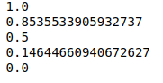
space = linspace(1, 0, 3)
for i in space:
    print(i)

space = cosinespace(1, 0, 5)
for i in space:
    print(i)

You can use the space and create a phase with them:

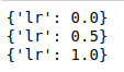
from poutyne import Phase

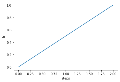
phase = Phase(lr=linspace(0, 1, 3))

# and iterate
for d in phase:
    print(d)

You can also visualize your phase:

import matplotlib.pyplot as plt
phase.plot("lr");

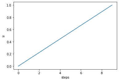
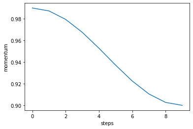
Phases can have multiple parameters:

phase = Phase(
    lr=linspace(0, 1, 10),
    momentum=cosinespace(.99, .9, 10),
)

phase.plot("lr");
phase.plot("momentum")

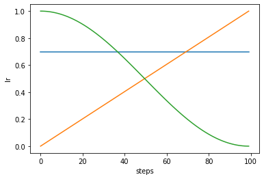
Visualize Different Phases¶

steps = 100

fig, ax = plt.subplots()
# Constant value
Phase(lr=linspace(.7, .7, steps)).plot(ax=ax)
# Linear
Phase(lr=linspace(0, 1, steps)).plot(ax=ax)
# Cosine
Phase(lr=cosinespace(1, 0, steps)).plot(ax=ax);

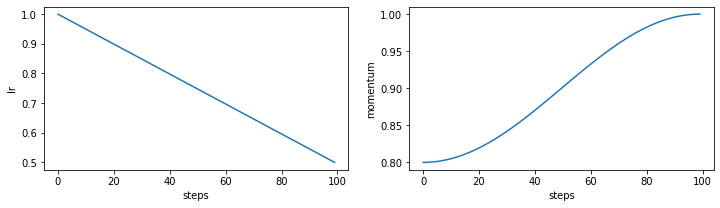
Visualize Multiple Parameters in One Phase¶

steps = 100
phase = Phase(lr=linspace(1, 0.5, steps), momentum=cosinespace(.8, 1, steps))

fig, axes = plt.subplots(1, 2, figsize=(12, 3))
phase.plot("lr", ax=axes[0])
phase.plot("momentum", ax=axes[1]);

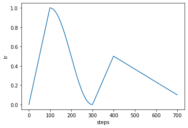
../_images/phase_multiple_parameters.png

Build Complex Policies From Basic Phases¶

You can build complex optimizer policies by chaining phases together:

from poutyne import OptimizerPolicy

policy = OptimizerPolicy([
    Phase(lr=linspace(0, 1, 100)),
    Phase(lr=cosinespace(1, 0, 200)),
    Phase(lr=linspace(0, .5, 100)),
    Phase(lr=linspace(.5, .1, 300)),
])

policy.plot();

Use Already Defined Complex Policies¶

It’s easy to build your own policies, but Poutyne contains some pre-defined phases.

from poutyne import sgdr_phases

# build them manually
policy = OptimizerPolicy([
    Phase(lr=cosinespace(1, 0, 200)),
    Phase(lr=cosinespace(1, 0, 400)),
    Phase(lr=cosinespace(1, 0, 800)),
])
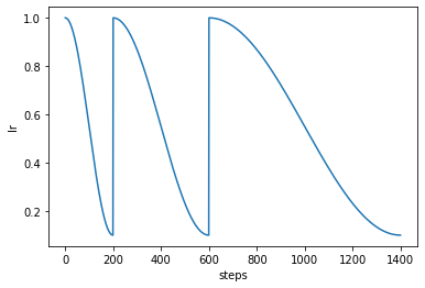
policy.plot()

# or use the pre-defined one
policy = OptimizerPolicy(sgdr_phases(base_cycle_length=200, cycles=3, cycle_mult=2))
policy.plot();

Pre-defined ones are just a list phases:

sgdr_phases(base_cycle_length=200, cycles=3, cycle_mult=2)

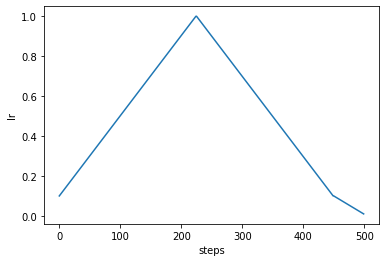
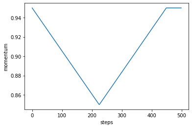
Here is the one-cycle policy:

from poutyne import one_cycle_phases

tp = OptimizerPolicy(one_cycle_phases(steps=500))
tp.plot("lr")
tp.plot("momentum");

Train CIFAR With the `policy` Module¶

Training Constants¶

But first, let’s set the training constants, the CUDA device used for training if one is present, we set the batch size (i.e. the number of elements to see before updating the model) and the number of epochs (i.e. the number of times we see the full dataset).

cuda_device = 0
device = torch.device("cuda:%d" % cuda_device if torch.cuda.is_available() else "cpu")

batch_size = 1024
epochs = 5

Load the Data¶

imagenet_mean = [0.485, 0.456, 0.406]
imagenet_std = [0.229, 0.224, 0.225]

train_transform = transforms.Compose([
    transforms.RandomHorizontalFlip(),
    transforms.ColorJitter(.3, .3, .3),
    transforms.ToTensor(),
    transforms.Normalize(imagenet_mean, imagenet_std),
])
valid_transform = transforms.Compose([
    transforms.ToTensor(),
    transforms.Normalize(imagenet_mean, imagenet_std),
])

root = "datasets"
train_dataset = datasets.CIFAR10(root, train=True, transform=train_transform, download=True)
valid_dataset = datasets.CIFAR10(root, train=False, transform=valid_transform, download=True)

train_loader = DataLoader(
    train_dataset,
    batch_size=batch_size,
    shuffle=True,
    num_workers=8
)
valid_loader = DataLoader(
    valid_dataset,
    batch_size=batch_size,
    shuffle=False,
    num_workers=8
)

The Model¶

We’ll train a simple ResNet-18 network. This takes a while without GPU but is pretty quick with GPU.

def get_network():
    model = resnet18(pretrained=False)
    model.avgpool = nn.AdaptiveAvgPool2d(1)
    model.fc = nn.Linear(512, 10)
    return model

Training Without the `policies` Module¶

network = get_network()
criterion = nn.CrossEntropyLoss()
optimizer = optim.SGD(network.parameters(), lr=0.01)

model = Model(
    network,
    optimizer,
    criterion,
    batch_metrics=["acc"],
    device=device,
)

history = model.fit_generator(
    train_loader,
    valid_loader,
    epochs=epochs,
)

Training With the `policies` Module¶

steps_per_epoch = len(train_loader)
steps_per_epoch

network = get_network()
criterion = nn.CrossEntropyLoss()
optimizer = optim.SGD(network.parameters(), lr=0.01)

model = Model(
    network,
    optimizer,
    criterion,
    batch_metrics=["acc"],
    device=device,
)

policy = OptimizerPolicy(
    one_cycle_phases(epochs * steps_per_epoch, lr=(0.01, 0.1, 0.008)),
)
history = model.fit_generator(
    train_loader,
    valid_loader,
    epochs=epochs,
    callbacks=[policy],
)

Interface of policy¶

About policy¶