Semantic segmentation using Poutyne
Note
See the notebook here
Run in Google Colab
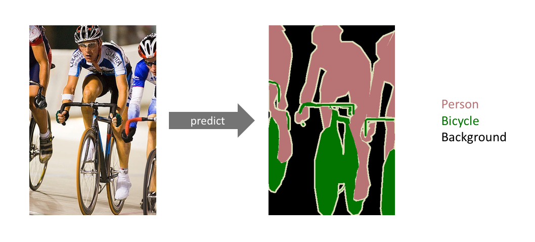
Semantic segmentation refers to the process of linking each pixel in an image to a class label. We can think of semantic segmentation as image classification at a pixel level. The image below clarifies the definition of semantic segmentation.
In this example, we will use and train a convolutional U-Net to design a network for semantic segmentation. In other words, we formulate the task of semantic segmentation as an image translation problem. We download and use the VOCSegmentation 2007 dataset for this purpose.
U-Net is a convolutional neural network similar to convolutional autoencoders. However, U-Net takes advantage of shortcuts between the encoder (contraction path) and decoder (expanding path), which helps it handle the vanishing gradient problem. In the following sections, we will install and import the segmentation-models-Pytorch library, which contains different U-Net architectures.
%pip install segmentation-models-pytorch
Let’s import all the needed packages and define some useful functions.
import os
import math
import matplotlib.pyplot as plt
import numpy as np
import torch
import torch.nn as nn
import torch.optim as optim
import torchvision.transforms as transforms
import torchvision.datasets as datasets
from torchvision.transforms.functional import InterpolationMode
import segmentation_models_pytorch as smp
import torchmetrics
from poutyne import Model, ModelCheckpoint, CSVLogger, set_seeds
from torch.utils.data import DataLoader
from PIL import Image


def replace_tensor_value_(tensor, a, b):
    tensor[tensor == a] = b
    return tensor


def plot_images(images, num_per_row=8, title=None):
    num_rows = int(math.ceil(len(images) / num_per_row))

    fig, axes = plt.subplots(num_rows, num_per_row, dpi=150)
    fig.subplots_adjust(wspace=0, hspace=0)

    for image, ax in zip(images, axes.flat):
        ax.imshow(image)
        ax.axis('off')

    return fig


# Color palette for segmentation masks
PALETTE = np.array(
    [
        [0, 0, 0],
        [128, 0, 0],
        [0, 128, 0],
        [128, 128, 0],
        [0, 0, 128],
        [128, 0, 128],
        [0, 128, 128],
        [128, 128, 128],
        [64, 0, 0],
        [192, 0, 0],
        [64, 128, 0],
        [192, 128, 0],
        [64, 0, 128],
        [192, 0, 128],
        [64, 128, 128],
        [192, 128, 128],
        [0, 64, 0],
        [128, 64, 0],
        [0, 192, 0],
        [128, 192, 0],
        [0, 64, 128],
    ]
    + [[0, 0, 0] for i in range(256 - 22)]
    + [[255, 255, 255]],
    dtype=np.uint8,
)


def array1d_to_pil_image(array):
    pil_out = Image.fromarray(array.astype(np.uint8), mode='P')
    pil_out.putpalette(PALETTE)
    return pil_out
Training constants
learning_rate = 0.0005
batch_size = 32
image_size = 224
num_epochs = 70
imagenet_mean = [0.485, 0.456, 0.406]  # mean of the imagenet dataset for normalizing
imagenet_std = [0.229, 0.224, 0.225]  # std of the imagenet dataset for normalizing
set_seeds(42)
device = torch.device('cuda' if torch.cuda.is_available() else 'cpu')
print('The current processor is ...', device)
Loading the VOCSegmentation dataset
The VOCSegmentation dataset can be easily downloaded from torchvision.datasets. This dataset allows you to apply the needed transformations on the ground-truth directly and define the proper transformations for the input images. To do so, we use the target_transfrom argument and set it to your transformation function of interest.
input_resize = transforms.Resize((224, 224))
input_transform = transforms.Compose(
    [
        input_resize,
        transforms.ToTensor(),
        transforms.Normalize(imagenet_mean, imagenet_std),
    ]
)

target_resize = transforms.Resize((224, 224), interpolation=InterpolationMode.NEAREST)
target_transform = transforms.Compose(
    [
        target_resize,
        transforms.PILToTensor(),
        transforms.Lambda(lambda x: replace_tensor_value_(x.squeeze(0).long(), 255, 21)),
    ]
)

# Creating the dataset
train_dataset = datasets.VOCSegmentation(
    './datasets/',
    year='2007',
    download=True,
    image_set='train',
    transform=input_transform,
    target_transform=target_transform,
)
valid_dataset = datasets.VOCSegmentation(
    './datasets/',
    year='2007',
    download=True,
    image_set='val',
    transform=input_transform,
    target_transform=target_transform,
)
test_dataset = datasets.VOCSegmentation(
    './data/VOC/',
    year='2007',
    download=True,
    image_set='test',
    transform=input_transform,
    target_transform=target_transform,
)

# Creating the dataloader
train_loader = DataLoader(train_dataset, batch_size=batch_size, shuffle=True, num_workers=2)
valid_loader = DataLoader(valid_dataset, batch_size=batch_size, shuffle=False, num_workers=2)
test_loader = DataLoader(test_dataset, batch_size=batch_size, shuffle=False, num_workers=2)
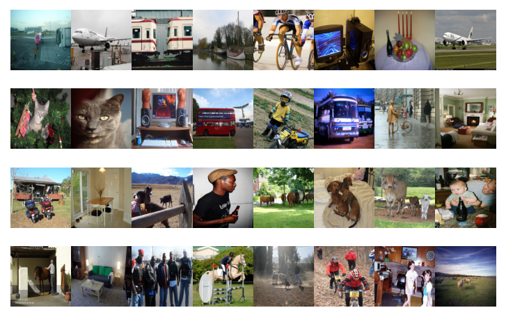
A random batch of the VODSegmentation dataset images
Let’s see some of the input samples inside the training dataset.
# Creating a VOC dataset without normalization for visualization.
train_dataset_viz = datasets.VOCSegmentation(
    './datasets/',
    year='2007',
    image_set='train',
    transform=input_resize,
    target_transform=target_resize,
)
inputs, ground_truths = map(list, zip(*[train_dataset_viz[i] for i in range(batch_size)]))

_ = plot_images(inputs)
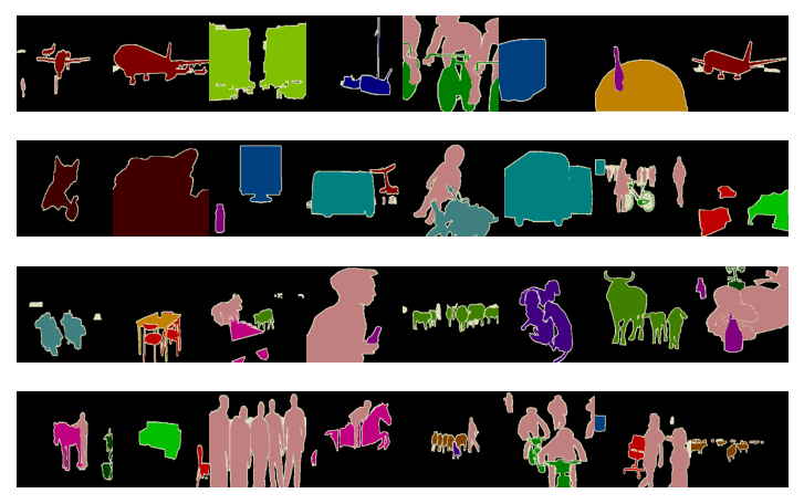
The ground-truth (segmentation map) for the image grid shown above is as below.
_ = plot_images(ground_truths)
It is worth mentioning that, as we have approached the segmentation task as an image translation problem, we use the cross-entropy loss for the training. Moreover, we believe that using the U-Net with a pre-trained encoder would help the network converge sooner and better. As this convolutional encoder is previously trained on the ImageNet, it is able to recognize low-level features (such as edge, color, etc.) and high-level features at its first and final layers, respectively.
# specifying loss function
criterion = nn.CrossEntropyLoss()

# specifying the network
network = smp.Unet('resnet34', encoder_weights='imagenet', classes=22)

# specifying optimizer
optimizer = optim.Adam(network.parameters(), lr=learning_rate)
As noticed in the section above, the ResNet-34-U-Net network is imported from the segmentation-models-pytorch library which contains many other architectures as well. You can import and use other available networks to try to increase the accuracy.
Training deep neural networks is a challenging task, especially when we are dealing with data with big sizes or numbers. There are numerous factors and hyperparameters which play an important role in the success of the network. One of these determining factors is the number of epochs. The right number of epochs would help your network train well. However, lower and higher numbers would make your network underfit or overfit, respectively. With some data types (such as images or videos), it is very time-consuming to repeat the training for different numbers of epochs to find the best one. Poutyne library has provided some fascinating tools to address this problem.
As you would notice in the following sections, by the use of callbacks, you would be able to record and retrieve the best parameters (weights) through your rather big number of epochs without needing to repeat the training process again and again. Moreover, Poutyne also gives you the possibility to resume your training from the last done epoch if you feel the need for even more iterations.
#callbacks

save_path = 'saves/unet-voc'

# Creating saving directory
os.makedirs(save_path, exist_ok=True)

callbacks = [
    # Save the latest weights to be able to continue the optimization at the end for more epochs.
    ModelCheckpoint(os.path.join(save_path, 'last_weights.ckpt')),

    # Save the weights in a new file when the current model is better than all previous models.
    ModelCheckpoint(os.path.join(save_path, 'best_weight.ckpt'),
                    save_best_only=True, restore_best=True, verbose=True),

    # Save the losses for each epoch in a TSV.
    CSVLogger(os.path.join(save_path, 'log.tsv'), separator='\t'),
]
Training
For training, we use the Jaccard index metric in addition to the accuracy and F1-score. The Jaccard index is also kwown as IoU is a classical metric for semantic segmentation.
# Poutyne Model on GPU
model = Model(
    network,
    optimizer,
    criterion,
    batch_metrics=['accuracy'],
    epoch_metrics=['f1', torchmetrics.JaccardIndex(num_classes=22, task="multiclass")],
    device=device,
)

# Train
_ = model.fit_generator(train_loader, valid_loader, epochs=num_epochs, callbacks=callbacks)
Calculation of the scores and visualization of results
There is one more helpful feature in Poutyne, which makes the evaluation task more easy and straight forward. Usually, computer vision researchers try to evaluate their trained networks on validation/test datasets by obtaining the scores (accuracy or loss usually). The evaluate methods in Poutyne provides you the loss and the metrics. In the next few blocks of code, you will see some examples.
loss, (acc, f1, jaccard) = model.evaluate_generator(test_loader)
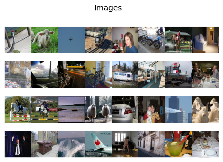
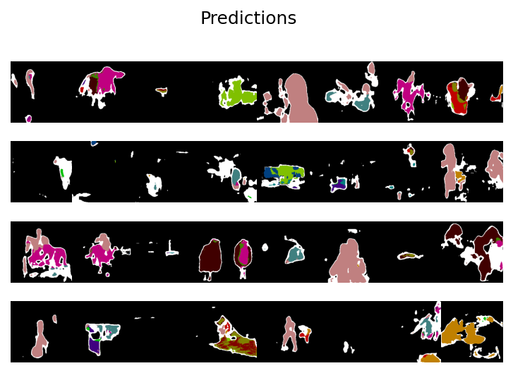
We show some of the segmentation results in the image below:
inputs, ground_truths = next(iter(test_loader))
outputs = model.predict_on_batch(inputs)
outputs = outputs.argmax(1)
outputs = replace_tensor_value_(outputs, 21, 255)
ground_truths = replace_tensor_value_(ground_truths, 21, 255)
plt_inputs = np.clip(inputs.numpy().transpose((0, 2, 3, 1)) * imagenet_std + imagenet_mean, 0, 1)
fig = plot_images(plt_inputs)
fig.suptitle("Images")
pil_outputs = [array1d_to_pil_image(out) for out in outputs]
fig = plot_images(pil_outputs)
fig.suptitle("Predictions")
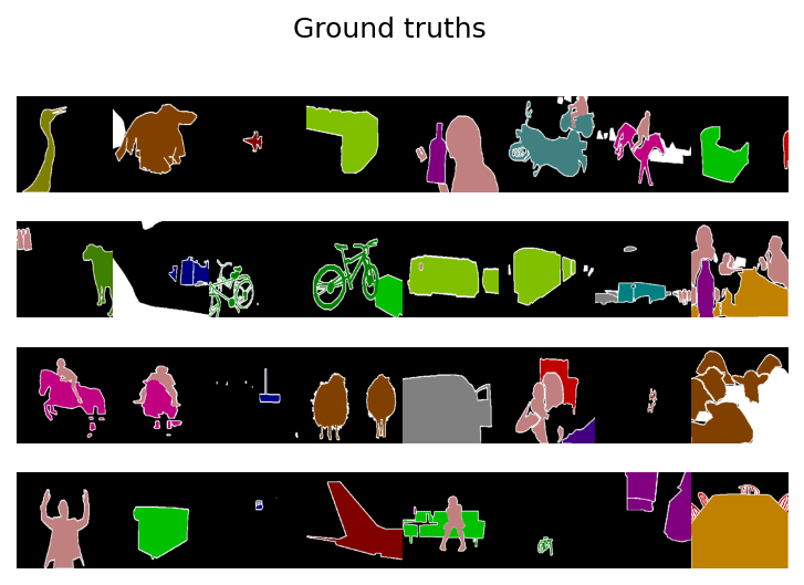
pil_ground_truths = [array1d_to_pil_image(gt) for gt in ground_truths.numpy()]
fig = plot_images(pil_ground_truths)
_ = fig.suptitle("Ground truths")
Last note
This example shows you how to design and train your own segmentation network simply. However, to get better results, you can play with the hyperparameters and do further finetuning to increase the accuracy.